Usage

chuchichaestli provides various modules that are essential throughout the creation of neural network models, from training to evaluation. It is meant as a repository of building blocks with which you can build your own neural network models.

Note

The framework integrates into the PyTorch ecosystem and as any artificial intelligence application is most efficiently used on GPU-based hardware.

We recommend combining the package with a configuration framework such as hydra. It can easily configure and instantiate chuchichaestli modules such as data loaders, neural network models, loss functions, and evaluation metrics.

Datasets

The data module provides dataset classes for common file types: HDF5Dataset, ImageDataset, NumpyDataset, and SafetensorsDataset. Each takes a single file or a wildcard pattern spanning an entire directory tree, and presents the whole collection as one indexable dataset. Accessed samples are cached as PyTorch tensors in shared memory up to a budget you set, with anything beyond it read from disk. With sufficient RAM, subsequent training epochs can be considerably accelerated.

For paired data, each class has a Zip* counterpart (ZipHDF5Dataset, ZipImageDataset, ZipNumpyDataset, and ZipSafetensorsDataset). Much like Python's built-in zip, these read several sources in lockstep and yield one sample per index as a tuple or dict, which is the usual setup for inputs and their labels or masks. Use ZipHDF5Dataset.from_groups(path, "image/*", "mask/*") to pair groups within the same file(s), or ZipDataset directly to combine datasets you have already built.

Example

Say, you have several HDF5 files with image datasets stored as

data
└── mnist_h5_tests
    ├── test_scenario_1
    │   └── mnist_test_1.h5
    ├── test_scenario_2
    │   └── mnist_test_2.h5
    ⋮
    └── test_scenario_13
        ├── test
        │   ├── mnist_test_test_00.h5
        │   └── mnist_test_test_01.h5
        ├── train
        │   ├── mnist_test_train_00.h5
        │   └── mnist_test_train_01.h5
        └── val
            ├── mnist_test_val_00.h5
            └── mnist_test_val_01.h5

then the following creates a dataset with 16 MiB of shared memory allocation to cache image tensors read from the H5 MNIST dataset (test scenario 13)

import torch
from chuchichaestli.data import HDF5Dataset

# select the training data in train
data_dir = "data/mnist_h5_tests/test_scenario_13/train"

# initialize the dataset
ds = HDF5Dataset(
    # the HDF5 files (wildcards * and ** work);
    # select all HDF5 files starting with 'mnist_test_' and ending with '.h5'
    path=f"{data_dir}/mnist_test_*.h5",
    # the HDF5 groups (wildcards * and ** work)
    groups="image/*",
    # data type is casted when accessed
    dtype=torch.float64,
    # allocate 16M as cache (for larger datasets, the rest is read from disk)
    cache="16M",
)

# Print summary info about the dataset
ds.info()

ZipHDF5Dataset reads multiple sample groups in parallel

import torch
from chuchichaestli.data import ZipHDF5Dataset

# select the training data in train
data_dir = "data/mnist_h5_tests/test_scenario_13/train"

zip_ds = ZipHDF5Dataset.from_groups(
    # the HDF5 files (wildcards * and ** work)
    f"{data_dir}/mnist_test_*.h5",
    # first HDF5 group
    "image/*",
    # second HDF5 group (acts as a "paired" source)
    "blurred_image/*",
    # each item is a plain (tensor_0, tensor_1) tuple
    zip_as="tuple",
    # both groups must have the same number of samples
    strict=True,
    # data type is casted when accessed
    dtype=torch.float32,
    # allocate 8M as cache for each dataset (for larger datasets,
    # the rest is read from disk)
    cache="8M",
)

print("First zip dataset")
zip_ds.datasets[0].info()
print("Second zip dataset")
zip_ds.datasets[1].info()

Procedural toy datasets

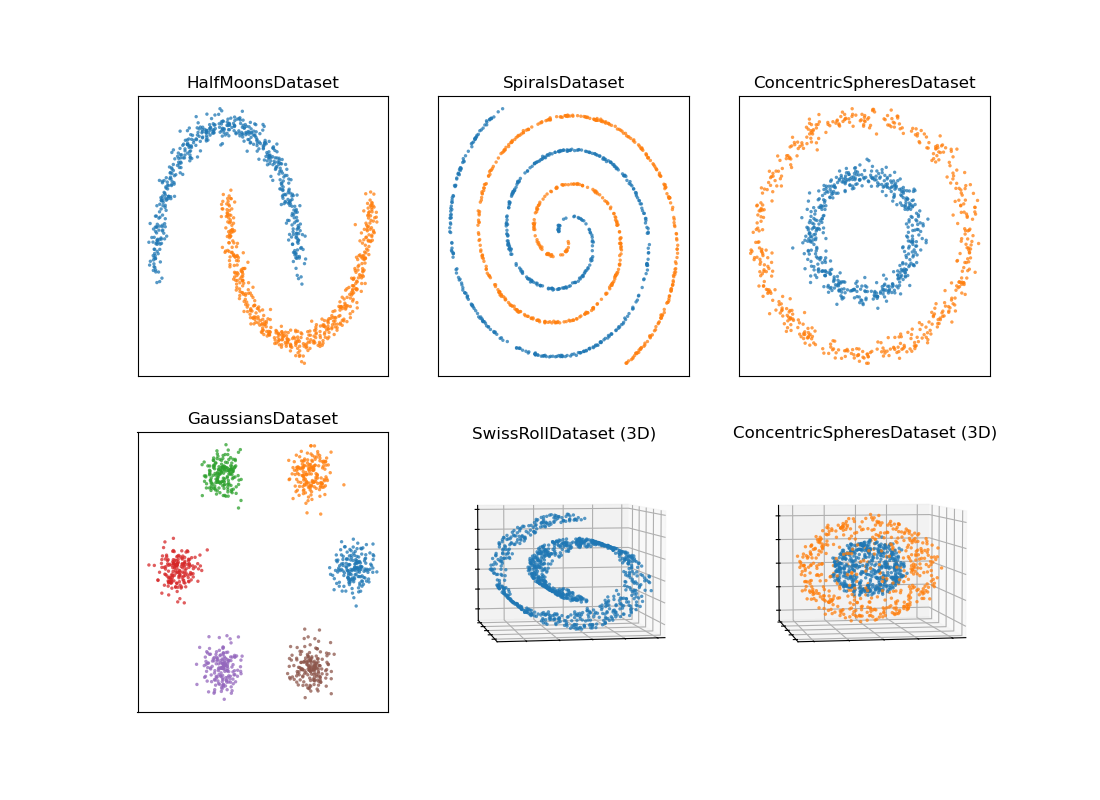
For quick experiments and sanity checks, the ProceduralDataset subclasses synthesize their samples on the fly instead of reading them from disk: HalfMoonsDataset, SpiralsDataset, CheckerboardDataset, RingsDataset, ConcentricSpheresDataset, GaussiansDataset, and SwissRollDataset. Each takes a sample count, a feature dimensionality, a noise level, and a seed for reproducibility, generating in pure PyTorch into the same shared-memory cache as the file-backed datasets.

from chuchichaestli.data import HalfMoonsDataset

# generate 1000 samples split into two half moons in 2D space
# preload the dataset into shared-memory cache before use
moons = HalfMoonsDataset(
    n_samples=1_000,
    noise=0.05,
    dim=2,
    seed=42,
    return_as="tuple",
    preload=True,
)
print(f"{moons}, shape={moons.shape}")
print(f"@index=0: sample shape={moons[0][0].shape}, label={moons[0][1]}\n")

The shapes are not restricted to the plane; raise dim to embed them in a volume instead.

from chuchichaestli.data import SwissRollDataset

# generate 1000 samples on a cylindrical spiral sheet embedded in 3D space
# preload the dataset into shared-memory cache before use
swissroll = SwissRollDataset(
    n_samples=1_000,
    noise=0.05,
    dim=3,
    seed=42,
    return_as="tuple",
    preload=True,
)
print(f"{swissroll}, shape={swissroll.shape}")
print(f"@index=0: sample shape={swissroll[0][0].shape}, label={swissroll[0][1]}\n")

Finally, you can also wrap your own generator function with generate_procedural_dataset.

Running examples/procedural_datasets.py renders all preset generators:

Models

The models module provides various neural network models ready to be instantiated such as UNet, VAE, or built with the components implemented in diffusion, models.attention, models.adversarial, and more.

These models are not pre-trained, meaning for proper functioning they have to be trained using appropriate data and objectives (loss functions).

Example

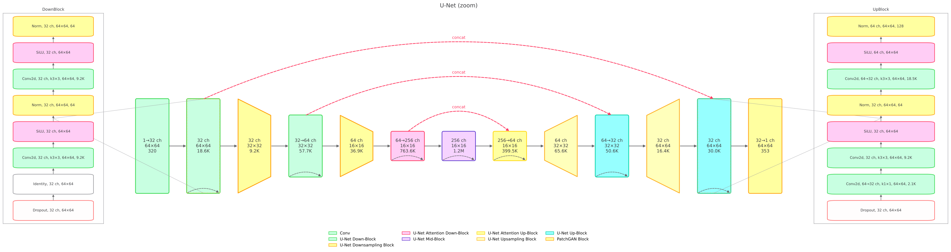
The U-Net architecture consists of an encoder-decoder structure with skip connections which ensure spatial information is passed through the network (even for higher compression levels). The building blocks of the U-Net can have various forms, but generally consist of convolutional layers. In this example, the U-Net's higher levels are purely convolutional, whereas the lowest levels include a mixture of attention and (transposed) convolutional layers.

from chuchichaestli.models.unet import UNet

model = UNet(
    dimensions=2,        # spatial dimensions
    in_channels=1,       # input image channels such as RGB or monochrome
    n_channels=32,       # channels of first hidden layer
    out_channels=1,      # output image channels such as RGB or monochrome
    down_block_types=("DownBlock", "DownBlock", "AttnDownBlock"),  # residual blocks and an attention block in the lowest level
    up_block_types=("AttnUpBlock", "UpBlock", "UpBlock"),  # an attention block in the lowest level and residual blocks
    block_out_channel_mults=(1, 2, 4),  # channel multipliers with each level
    res_act_fn="silu",   # SiLU activations
    res_dropout=0.4,     # dropout for residual blocks
    attn_n_heads=1,      # number of attention heads per block,
    skip_connection_action="concat",    # skip connections are concatenated in decoder
)

summary provides a torchinfo-style text table (no extra dependency) that allows for detailed inspection of any model

from chuchichaestli.utils.info import summary

INPUT_SHAPE = (1, 1, 64, 64)
print(
    summary(
        model,
        input_shape=INPUT_SHAPE,
        depth=3,
        columns=("input", "output", "kernel", "params", "mult_adds"),
    )
)

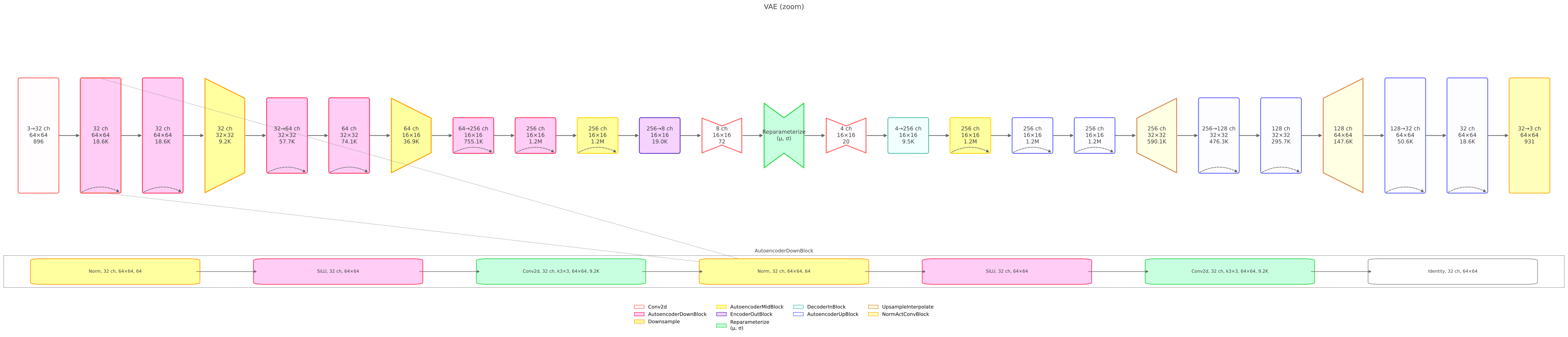
Similarly, you can build other models such as a Variational Auto-encoder (VAE) using autoencoding-specific building blocks. The model is quite similar to a U-Net, but misses skip connections and instead includes a stochastic regularization prior in the lowest layer (the latent)

from chuchichaestli.models.autoencoder import VAE, VAEDecoder, VAEEncoder

encoder = VAEEncoder(
    dimensions=2,
    in_channels=3,
    n_channels=32,
    out_channels=4,
    down_block_types=("AutoencoderDownBlock",) * 3,
    block_out_channel_mults=(1, 2, 4),
    num_layers_per_block=2,
    mid_block_types=("AutoencoderMidBlock",),
)
decoder = VAEDecoder(
    dimensions=2,
    in_channels=4,
    n_channels=encoder.bottleneck_channels,
    out_channels=3,
    up_block_types=("AutoencoderUpBlock",) * 3,
    block_out_channel_mults=(1, 2, 4),
    num_layers_per_block=2,
    mid_block_types=("AutoencoderMidBlock",),
)
model = VAE(encoder, decoder)

Autoencoders take their two components as arguments, so an encoder and a decoder can be configured, reused, or swapped independently. When you would rather describe the architecture in one call, build assembles both components for you: arguments shared by them stay flat, while anything specific to one component goes into encoder_args or decoder_args, whose keys are the parameter names of Encoder and Decoder. Keys you leave out fall back to the defaults of the component itself, which is where each variant keeps its architecture: VAE builds a VAEEncoder/VAEDecoder pair whose encoder doubles the latent channels, and DCAE a DCEncoder/DCDecoder pair of deep-compression blocks.

from chuchichaestli.models.autoencoder import DCAE, DCDecoder, DCEncoder

model = DCAE.build(dimensions=3, latent_dim=32)
# equivalently, with the components built by hand
encoder = DCEncoder(dimensions=3, out_channels=32)
decoder = DCDecoder(
    dimensions=3, in_channels=32, n_channels=encoder.bottleneck_channels
)
model = DCAE(encoder, decoder)

Both forms map directly onto a configuration framework such as hydra, either as nested groups you can override one at a time, or as a single flat group

model:
  _target_: chuchichaestli.models.autoencoder.DCAE
  encoder:
    _target_: chuchichaestli.models.autoencoder.DCEncoder
    dimensions: 3
    out_channels: 32
  decoder:
    _target_: chuchichaestli.models.autoencoder.DCDecoder
    dimensions: 3
    in_channels: 32
    n_channels: 1024
# or
model:
  _target_: chuchichaestli.models.autoencoder.DCAE.build
  dimensions: 3
  latent_dim: 32

Visualization

The visualization utilities turn a model into a schematic. A backend-agnostic semantic graph (build_ir) understands the architecture hierarchy, components (encoder/bottleneck/decoder), spatial levels, blocks, and layers, including skip and residual connections. Architecture-aware adapters handle U-Nets and autoencoders (VAE/VQVAE/DCAE); any other PyTorch model (e.g. a torchvision ResNet or ViT) falls back to a generic adapter that mirrors the module tree.

Two entry points consume the graph: - matplotlib_diagram — vector figures (PDF/SVG/PNG); requires the optional viz extra. - mermaid_diagram — quick markdown/web diagrams.

Matplotlib figures

Matplotlib diagrams are most versatile and are recommended as starting point to produce publication-ready illustrations. level selects the abstraction (0=components, 1=levels, 2=blocks, 3=layers). label_fields chooses what each node shows (name, channels, kernel, resolution, params); color_by chooses what the fill colours and legend encode (component, type, or name); node_size is small/medium/large.

from pathlib import Path
from chuchichaestli.utils.visualization import (
    matplotlib_diagram,
    mermaid_diagram,
    ZoomSpec,
)

DIR = Path(__file__).resolve().parent
LEVEL_LABELS = ("channels", "resolution", "params")

for level in range(4):
    matplotlib_diagram(
        model,
        level=level,
        input_shape=INPUT_SHAPE,
        node_size="small" if level >= 3 else "medium",
        label_fields=("name",) + LEVEL_LABELS if level == 1 else LEVEL_LABELS,
        color_by="component" if level <= 1 else "type",
        title=f"U-Net (level {level})",
    ).save(DIR / f"unet_level{level}.svg")

An exemplary zoom callout expands a block into its layers: zoom=True auto-picks a representative block, or pass a node id / ZoomSpec. zoom_loc places the inset (right/left/top/bottom, the four corners, or center); pass a list of ZoomSpecs to draw several at once.

from chuchichaestli.utils.visualization import ZoomSpec

matplotlib_diagram(
    model,
    level=2,
    zoom=[
        ZoomSpec("model/encoder/level0/block0", loc="left", size=0.15),
        ZoomSpec("model/decoder/level2/block4", loc="right", size=0.2),
    ],
    input_shape=INPUT_SHAPE,
    label_fields=("channels", "resolution", "params"),
    color_by="type",
    title="U-Net (zoom)",
).save(DIR / "unet_zoom.svg")

The same block-level view of a VAE has no skip arcs and swaps the U-Net's concatenation for a latent bottleneck (the hourglass node); here a single zoom inset expands an encoder block into its layers:

Mermaid diagrams

The Mermaid backend compiles a .mmd file that can be imported into a mermaid web-editor (e.g. mermaid.live), where individual nodes can be dragged to fine-tune the layout. The overall flow is controlled with direction/group_direction, and group_by nests per-block subgraphs inside the encoder/decoder subgraphs; skip connections render as dashed edges.

from chuchichaestli.utils.visualization import mermaid_diagram

diagram = mermaid_diagram(
    model, input_shape=INPUT_SHAPE, group_by=["encoder_decoder", "block"], max_depth=4
)

diagram.save(DIR / "unet.mmd")

Runnable end-to-end scripts for a U-Net, a VAE, a PatchGAN discriminator, and torchvision models (ResNet + ViT) live in examples/.

Metrics

The metrics module provides various metrics and losses to measure and compare image quality of fake and real samples. In contrast to many other image quality metric libraries, chuchichaestli's only dependency for this module (besides torch itself) is torchvision. This makes chuchichaestli still very lightweight and avoids package conflicts during installs.

Example

All metrics share the same interface: .update registers a batch into the aggregate state while iterating over the evaluation set, and .compute reduces that aggregate to a value once the loop is done.

A toy stand-in for a model and its evaluation set:

import torch
from chuchichaestli.metrics import MSE, PSNR, SSIM

torch.manual_seed(42)
batch_size, num_channels, width, height = 4, 3, 128, 128


def evaluation_batches(n_batches: int = 8):
    """Stand-in for a real evaluation loop over a model and a dataset.

    Yields (data, prediction) pairs, i.e. the target images alongside the
    imperfect reconstructions a model would produce for them.
    """
    for _ in range(n_batches):
        data = torch.rand(batch_size, num_channels, width, height)
        prediction = (data + 0.05 * torch.randn_like(data)).clamp(0, 1)
        yield data, prediction

metrics = [
    MSE(),
    PSNR(min_value=0, max_value=1),
    SSIM(min_value=0, max_value=1, kernel_size=7, kernel_type="gaussian"),
]

# `update` accumulates state across the entire evaluation set...
for data, prediction in evaluation_batches():
    for metric in metrics:
        metric.update(data, prediction)

# ...while `compute` reduces that aggregate once, after the loop
for metric in metrics:
    print(f"{type(metric).__name__:<4s} = {metric.compute():.4f}")
    metric.reset()

Note the argument order: update takes the observed data first, the prediction second. FID shares the interface but compares feature distributions instead of pixels, keeping real and fake statistics apart; its default InceptionV3 extractor is downloaded on first use.

from chuchichaestli.metrics import FID

# FID scores feature distributions instead of pixels, so real and fake images
# are aggregated into separate statistics
fid = FID()
for data, prediction in evaluation_batches():
    fid.update(data=data, prediction=prediction)

print(f"FID  = {fid.compute():.4f}")